GWRech
Groundwater Recharge, Groundwater Discharge
and Change in Aquifer Storage
Estimation Tool
-
1. About GWRech
GWRech is an online tool that allows for estimation of daily groundwater recharge, groundwater discharge and the change in aquifer storage using an adaptation of the Water Table Fluctuation (WTF) method for multi-layered systems. The tool requires user provided aquifer (or material) specific yield and daily water table elevations. The tool is free to use and does not require user registration.
GWRech has been developed through a collaborative research effort between Canadian Rivers Institute (CRI), University of New Brunswick (UNB), Agriculture and Agri-Food Canada (AAFC) and Environment and Climate Change Canada (ECCC). GWRech is the result of a larger research effort aimed at evaluating the effects of agricultural production systems on groundwater and surface water quantity and quality. GWRech is part of Hydrology Tool Set (HTS; https://portal.hydrotools.tech). HTS includes additional applications, such as SepHydro (daily baseflow / hydrograph separation; 11 methods), ETCalc (daily potential, reference and actual evapotranspiration estimation; 8 methods), SWIB (daily estimation of soil water stress, crop water deficit, irrigation requirement and its impact on aquifer storage, water budget components), SNOSWAB (daily estimation of water balance terms, including snowfall, snowmelt, snowpack, soil water content, evapotranspiration, drainage, infiltration, surface runoff), TotPrePart (partitioning of daily total precipitation into snowfall and rainfall) and FLEX-WQI (estimation of water quality state via water quality indexes).
If you used GWRech, please include the following citation(s) in your publication(s):
Danielescu S (2025) GWRech - An online tool for estimating groundwater recharge, groundwater discharge and change in aquifer storage. Reference Manual.
Available at https://gwrech.hydrotools.tech. -
2. Background
Groundwater recharge (also known as deep drainage or deep percolation) is a hydrological process through which aquifers receive water and thus allows for replenishing of groundwater resources. Most typically, groundwater recharge is related to the downward movement (via. infiltration and percolation) of water from the surface of the ground to the aquifer and is generally a result of natural processes such as rain and snowmelt, but can also be artificially induced. Conversely, groundwater discharge represents the loss of water from the aquifer, a process through which water from the aquifer flows for example to streams, lakes and oceans. The difference between groundwater recharge and groundwater discharge represents the change in aquifer storage. Groundwater recharge and groundwater discharge are extremely important for appropriate management of groundwater systems and are key components of many water resource studies aimed at understanding the dynamics of aquifer water storage. Thus, their estimation is important for studies involving for example groundwater quantity and contaminant transport modelling, irrigation, climate change, saltwater intrusion in coastal areas, weathering of rock material, etc.
The Water Table Fluctuation (WTF) method, widely used in hydrogeological studies (e.g., Healy and Cook, 2002; Scanlon and Healy, 2002; Coes et al., 2007; Labrecque et al., 2010) allows for estimation of groundwater recharge in unconfined aquifers based on the specific yield of the aquifer (or material) and the changes in water table elevation. Daily groundwater recharge is calculated using the following equation:
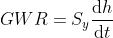
GWR - Groundwater recharge (mm)
Sv - Specific yield (m3/m3) dh - positive change in water table elevation between two consecutive days (mm)
dt - change in time (day)
Conversely, daily groundwater discharge is calculated using the following equation:

GWD - Groundwater discharge (mm)
Sv - Specific yield (m3/m3) dh - negative change in water table elevation between two consecutive days (mm)
dt - change in time (day)
The change in aquifer storage is calculated as the sum between groundwater recharge (positive values) and groundwater discharge (negative values) using the following equation:

ΔS - Change in aquifer storage (mm)
GWR - Groundwater recharge (mm)
GWD - Groundwater discharge (mm)
Specific yield (also known as drainable porosity) is defined as the ratio of the volume of water that a saturated rock or soil will yield by gravity to the total volume of the rock or soil. Specific yield can be estimated through various methods; however, if these estimates are not available, specific yield values for various soil and rock types are available in literature.
The change in water table elevation, defined as the difference in water table elevation between two consecutive days, is used for determining the presence of groundwater recharge and discharge processes. Thus, groundwater recharge is considered to occur if the change is positive and groundwater discharge is considered to occur if the change is negative.
WTF method has the advantage of being a simple and easy to use method. The values of groundwater recharge and discharge estimated with this method are representative for a wide range of spatial scales, provided the water levels are representative for the aquifer as a whole, and thus, WTF method provides a distinct advantage over point measurement approaches (Healy and Cook, 2002).
The WTF method has been adapted in the GWRech tool to allow for estimation of groundwater recharge and groundwater discharge in multi-layered systems. Thus, the user can define the properties (e.g., thickness and specific yield) of up to 30 layers and, depending on the position of the user-provided water table elevation, GWRech will calculate for each day the groundwater recharge (or the groundwater discharge) based on the properties (i.e., specific yield) of the layer in which the water table is positioned.
GWRech can be used for any location for which input data is provided by the user. The tool includes routines for validating the output when user-provided calibration data is supplied. The web-based tool provides various data visualization, analysis and output (i.e., export) options through a streamlined process and a user-friendly interface. The Test Data set allows users to test the various routines and familiarize themselves with the tool.
GWRech has a broad range of applicability and can be used for standalone analyses of groundwater recharge, groundwater discharge and change in aquifer storage; for generation of critical data for external models that allow for uploading of user-provided groundwater recharge or groundwater discharge; or for educational purposes to demonstrate the significance and the dynamics of groundwater recharge and groundwater discharge processes.
-
3. User Guide
At the top, a contextual menu provides access to the various modules of the tool. The modules can be accessed progressively, in the following order: 1) Home (Information module); 2) Input Data (Data entry module); and 3) Analysis (Calculation module). Once the calculations of a module are completed, the user can advance to the next module and can also return to the respective module at any time during the session. Menu tabs are available for both the data entry (i.e., Info, Load Data, Graphical View, Table View and Export Input Data for the Input Data module) and calculation (i.e., Info, Analysis, Graphical View, Table View and Export) modules. Additional buttons (i.e., UCD and Reset Data) appear in the contextual menu once the Input Data is loaded to the tool.
GWRech uses daily timestep for both input and output data and includes a series of averaging options for displaying and exporting data (i.e., monthly, seasonal [meteorological and growing season], yearly). GWRech also calculates and allows for displaying of input and output data using as a "typical year daily" timeseries (i.e., daily multi-year averages for each day of the year available in the input and output files) when the analysis is carried out for a period longer than one year. The daily values for the typical year can also be averaged by the tool over monthly, seasonal [meteorological and growing season], and yearly periods. Daily typical and monthly averaging intervals are recommended for inspecting and analyzing "average" conditions when the datasets cover longer periods of time (several years).
In the following sections the options available under the various modules of the tool, together with details about the output data, calibration procedure and data inspection, visualization and export are presented in separate subsections.
3.1. Quick start
In order to run GWRech the user has to complete the following steps:
-
Load Data: provide required data or use the provided test data [Input Data module];
-
Perform groundwater recharge, groundwater discharge and change in water storage calculations: enter required coefficients and select Run Analysis [ANALYSIS module – Analysis tab]. The calibration of the tool is conducted by adjusting the coefficients available on this page (i.e., specific yield; lower and upper elevations for each layer) in conjunction with the information displayed in the Calibration overlay window launched by using the Run Analysis button;
-
Investigate Results and Export Data: review GWRech output from each module [Table View and/or Graphical View] and export results [Export Data button available under each data entry and calculation modules or the CSV button available under the Stats and Calibration Stats of the Graphical View or under the Table, Stats and Calibration Stats of the Table View].
The steps required for using this tool are described in more detail below.
3.2. Home Module
This module contains information related to the development, methodology and use of GWRech. Under each of the input and calculation modules an Info tab is available, where general information relevant to the respective module is provided.
3.3. Input Data Module
The first step in conducting an analysis is to upload the input data file to be used by GWRech. The users can run GWRech either by using the test dataset or by uploading a new dataset.
For testing GWRech and better understanding how the various components of the tool operate, the user can upload the test data set provided by clicking on "Try the tool using the test dataset" button. The test dataset contains three years of weather and user calibration data (UCD). Test dataset UCD data consists of groundwater recharge (mm; UCD1; corresponding to GWRech Groundwater Recharge output parameter; UCD1 estimated from groundwater levels measured in research wells at AAFC Harrington Experimental Farm, Prince Edward Island, Canada), groundwater discharge (mm; UCD2; corresponding to GWRech Groundwater Discharge output parameter; UCD2 estimated from groundwater levels measured in research wells at AAFC Harrington Experimental Farm, Prince Edward Island, Canada), and soil water content (m/m; UCD3; UCD3 measured at Agriculture and Agri-Food Canada [AAFC] Harrington Experimental Farm, Prince Edward Island, Canada).
For using GWRech, the users need to upload daily timeseries. The tool accepts source data sets in Comma Separated File (csv) format. The users can use the "Download Sample File" button located on the Upload User Data Page (Load Data) or the "Export Input Data - Daily" menu to obtain a correctly formatted input file that can be used as a model for populating the input data file with user data. The "Export Input Data - Daily" menu becomes available after the test or a user dataset is loaded. The user input file can be uploaded to GWRech by using the "Upload user data" button. GWRech allows uploading of files with maximum 7500 rows (~20 years of daily data). It is recommended to split the input data set in blocks of 20 years daily timeseries when the intent is to analyze longer time periods. It should be noted that the tool cannot accommodate missing data (i.e., blank rows in required data columns) or erroneous data entries, and hence it is recommended that the integrity of the source data is verified before uploading. An error message will be displayed, and the user will be redirected to the Load Data page if inconsistencies are detected in the user file.
The input data file consists of a tabular file, with the first row dedicated to the parameter names, 1 column dedicated to calendar date, 1 column dedicated to required input data (WTELEV - Water Table Elevation; m.a.s.l. – meters above sea level) and 3 columns reserved for optional user calibration data (UCD1 to UCD3). The required input data columns have to contain values in all rows, while the optional data columns (i.e., UCD) can be left blank if data is not available. If UCD data is provided, then all the rows in the respective column(s), except for the column headings, must contain numeric values. UCD data sets are not restricted to certain parameters and can include time series for any parameter that the user intends to use for comparing with the output from GWRech. Although UCD data is optional, it provides critical information for adjusting the various coefficients of the tool during the calibration procedure. Examples of calibration time series datasets include groundwater recharge and discharge obtained with other methods, soil water content, stream discharge, infiltration, evapotranspiration, etc.
The number of columns, data format and the units of the various timeseries required for the input file are shown in the table below.
Columns DATE WTELEV UCD (max. 3 columns) Units yyyy-mm-dd m user choice Values eg. 2021-12-24 -1000 to 8000 user choice
Notations:
-
Required data:
DATE - use yyyy-mm-dd format;
WTELEV - daily water table elevation; -
Optional data:
UCD - user calibration data (up to three columns; leave blank if no data is available)
Notes:
-
The tool requires daily data
-
The user input data file has to be uploaded using a file with 1 column dedicated to calendar date, 1 column dedicated to required input data (WTELEV) and 3 columns reserved for optional user calibration data (UCD1 to UCD3)
-
Use the first row of the data set for column headings
-
GWRech includes several input data integrity and quality check routines; however, the user is advised to thoroughly check the input dataset before uploading it to the tool to minimize the risk for erroneous output
Once the input dataset is loaded to GWRech via either the "Try the tool using the test data set" or "Upload user data" button an overlay window appears (i.e., "Select the UCD averaging method") asking the user to specify the method used for calculation of monthly values for each UCD timeseries (i.e., averaging vs. summation). Once this step is completed a new button ("UCD") is added to the right of the Input Data tab at the top of the page and the view switches to Graphical View. The UCD menu available at the top of the page allows the user to change the method for the calculation of monthly values for each UCD at any time. See section 3.7. for instructions regarding the inspection of datasets using tables and graphs as well as for the various options available for exporting the data.
Once the loading and inspecting of the input data is completed the user can click on the ANALYSIS menu entry at the top of the page to advance to the calculation module.
3.4. Analysis Module
On the Analysis Tab the user must first provide the coefficients required by the tool in the "Vertical distribution of specific yield" and "Calibration mapping" sections of the page. The values of the coefficients can be entered manually using the collapsible menus available under the Analysis Tab or can be uploaded as a set using the "Import configuration file" button. Once specified, the values of the coefficients can be checked using the "Validate" button at the bottom of the page. An error message is displayed if the coefficients include blank, out of range or incorrect format data. "Run Analysis" button replaces the "Validate" button if no errors in coefficient values are found during the validation. The configuration file can be downloaded using the "Export Configuration File" button under the Analysis Tab (including either default values of the coefficients if the first tool run has not been completed or values of the coefficient as set for the last available run of the tool if the analysis has been completed at least once) or by using "Export Configuration" in the "Export Results" menu (available after one successful run of the module). If needed, the users can also reset all the values of the coefficients to default values by using the "Reset to Default" button available at the bottom of the page in the Analysis tab.
In the "Vertical distribution of specific yield" section of the page the user have to enter the lower and upper bound elevations as well as the specific yield for each layer of the domain. The number of layers can be expanded or reduced using the "+" or "-" buttons at the left of coefficient fields. Lower and upper bound elevations values between -1000 and 8000 m.a.s.l. (meters above sea level) are allowed. Of note, use of depths instead of elevations will result in erroneous results. When entering values in the elevation fields, the user have to check that the depth intervals do not overlap and the lower bound elevation is smaller than the upper bound elevation for each layer. For specific yield, the values have to be between 0 and 1 and the units currently used are m3/m3. For reference, the specific yield values can be converted to percentages if they are multiplied by 100 (e.g., 0.1 m3/m3 is equal to 10%).
In the "Calibration mapping" section of the page the users have to select the pairs of tool output and user calibration data that will be used during the calibration of the tool. The "Calibration Mapping" fields can be ignored if the UCD data is not available in the Input Data file.
GWRech starts the calculations once the values of the required coefficients are set and the user clicks on the Run Analysis button at the bottom of the page.
All values entered on this page can be subsequently adjusted during the calibration procedure, with calibration being considered final once no further improvement in the output fitness is observed. See section 3.6 for instructions regarding the calibration of the tool and section 3.7. for instructions regarding the inspection of datasets using tables and graphs as well as for the various options available for exporting the data.
3.5. Output Timeseries
The output from GWRech is shown in the table below.
NAME DESCRIPTION Index Indicates the position of a specific record (line) in the timeseries. Change in WT Elev. (mm) Change in Water Table (WT) Elevation. For daily timestep the values in this column are calculated as the difference between Water Table (WT) Elevations for two consecutive days (i.e. ΔWT Elev. = WT Elevt+1 - WT Elevt). For all other averaging intervals this is calculated as the difference between the last day and the first day in the interval (e.g., for monthly this is calculated as the difference between the water table elevation on the last day of the month and the water table elevation on the first day of the month). The units for ΔWT Elev. are mm. Groundwater Recharge (mm) This is the amount of groundwater recharge and is always calculated using the daily timestep. When the data is displayed using averaging intervals other than daily, this is calculated as the sum of daily recharges (i.e., recharge is calculated only for the days when ΔWT Elev. is positive). The units for Groundwater Recharge are mm. To obtain the volume of recharge for a given area the user has to multiply this value with the land area of interest. Groundwater Discharge (mm) This is the amount of groundwater discharge and is always calculated using the daily timestep. When the data is displayed using averaging intervals other than daily, this is calculated as the sum of daily discharges (i.e., discharge is calculated only for the days when ΔWT Elev. is negative). The units for Groundwater Discharge are mm. To obtain the volume of discharge for a given area the user has to multiply this value with the land area of interest. Change in aquifer storage (mm) The change in aquifer storage is calculated on a daily basis as the product of ΔWT Elev. and specific yield. When positive, this indicates occurrence (i.e., dominance) of groundwater recharge, and when negative occurrence (i.e., dominance) of groundwater discharge. When the data is displayed using averaging intervals other than daily, this is calculated as the sum of daily changes, and thus, it shows the "net" change in storage over the respective averaging interval. The values calculated in this column are assigned to the Groundwater Recharge if positive and to Groundwater Discharge columns if negative. Consult sections 2 and 4 for additional details.
3.6. Calibration Procedure
Calibration of the tool is performed via the Analysis tab of ANALYSIS module and is available only when UCD data is included in the Input data file. Calibration is conducted by first pairing the datasets from the output of the tool with the user calibration data (UCD) using the “Calibration mapping” menu available under the “Analysis” tab. Once the pairing is completed, the user can proceed to adjust coefficients, validate the data (“Validate” button at the bottom of the Analysis page) and run the tool (i.e., “Run Analysis” button at the bottom of the Analysis tab page) and inspect the tool output in the subsequent Calibration overlay window. The fitness of the output for various timesteps and averaging intervals can be inspected in the Calibration overlay window via graphs as well as bivariate statistics. If the calibration is considered unsatisfactory the user can return to the Analysis menu (i.e., “Return” button), adjust the various coefficients of the tool and rerun the analysis. If the calibration is considered satisfactory the user can complete the calculations by proceeding to the next step (i.e., “Proceed to results” in the Calibration Overlay window).
To aid with data inspection and assessment of the fitness of the output data, GWRech includes several univariate and bivariate statistics. Univariate statistics, including, average, minimum, maximum and standard deviation are calculated separately for the input (i.e., user provided calibration data) and tool output time series. The graphs and the univariate statistics can be used for example for comparing the general trends, the range of values and the amplitude of variations in both data sets. The bivariate statistics include the coefficient of determination (R2), root mean square error (RMSE) and the normalized root mean square error (NRMSE). NRMSE is calculated by using the average, the interquartile range or the differences between maximum and minimum (see definitions below). The bivariate statistics are used for evaluating the fitness of the output, by providing a measure of the differences between the values calculated by the tool and the user provided calibration data (i.e., UCD). The equations used for calculating each bivariate statistic are shown below.
Eq 2. - Coefficient of determination
R2 - coefficient of determination
xi - value for observed data on day i
yi - value for modelled data on day i
xmean - mean of observed data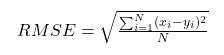
Eq 3. - Root mean square error
RMSE - Root mean square error
N - number non-missing data points
xi - value for observed data on day i
yi - value for modelled data on day i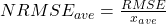
Eq 4. - Normalized root mean square error average
NRMSEave - normalized root mean square error calculated using the average value of measured data
RMSE - root mean square error
xa - average value of observed data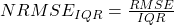
Eq 5. - Normalized root mean square error IQR
NRMSEIQR - normalized root mean square error calculated using minimum and maximum values of measured data
RMSE - root mean square error
IQR - interquartile range of the observed data; IQR = Q3-Q1,
with Q3 = CDF-1(0.25), Q1 = CDF-1(0.75),
where CDF is the quantile function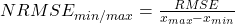
Eq 6. - Normalized root mean square error min/max
NRMSEmin/max - normalized root mean square error calculated using minimum and maximum values of measured data
RMSE - root mean square error
xmax - maximum value for observed data
xmin - minimum value for observed data
It is recommended that the calibration is conducted by changing one coefficient at a time over a selected range of values. When no further improvement is observed in the fitness of GWRech output the user can advance to adjusting the values of the next coefficient. The values of the various coefficients can be considered final once no further improvement in the fitness of the GWRech output is observed. Currently, only calibration by trial and error is available, however the integration of an autocalibration routine is in planning stages.
3.7. Data inspection, visualisation and export
Inspection of data via graphical and tabular views can be conducted via the Graphical View, Table View and Export Data menu entries that become available in the Input Data module once the input dataset is loaded to GWRech. These menu entries are also available under each ANALYSIS module and allow the user to evaluate the output for each of these modules.
Graphical View allows for plotting of input or output data using various time steps and intervals available via a drop-down menu. The parameters that can be displayed are available in the selection pane located to the right of the plot. Each parameter can be displayed on the primary (left) Y axis or on the secondary (right) Y axis by clicking on the toggle placed at the right of the selection pane. Additional options for customizing the plot become visible in the top right corner when the mouse pointer is placed above the plot. These options include zoom, auto scale, reset axes, show data point labels, download plot, etc. Univariate statistics (average, minimum, maximum, standard deviation) for selected timeseries and bivariate statistics (R2, RMSE, NRMSEave, NRMSEIQR, NRMSEmin/max) for inspecting the fitness of the tool output are available under the Stats and Calibration Stats tabs, respectively. These statistics are available either for the entire dataset ("Show Complete Dataset Stats" button) or for a selected subset ("Show stats by Interval" button). The tables shown on the statistics pages can be exported individually by using the corresponding CSV button located to the right of the page.
Table View allows the user to display data in tabular format using various time steps and intervals. The user can also change the number of lines, filter data based on date or adjust the starting date of the data that is displayed. In the initial Table View, the columns displayed by default are limited to "key" parameters, however the user can change the selection of the parameters to be displayed by selecting the parameters listed above the table. In the respective list, the parameters that are displayed in the table are shown in filled boxes, while the ones that are omitted are included in clear boxes. The "key" parameters are shown in red font when not selected to be displayed. Similar to the Graphical View, univariate statistics (average, minimum, maximum, standard deviation) for selected timeseries and bivariate statistics (R2, RMSE, NRMSEave, NRMSEIQR, NRMSEmin/max) for inspecting the fitness of the output are available under the Stats and Calibration Stats tabs, respectively. These statistics are available either for the entire dataset ("Show Complete Dataset Stats" button) or for a selected subset ("Show stats by Interval" button). The tables shown on the statistics pages can be exported individually by using the corresponding CSV button located to the right of the page.
The Export Data tab offers additional options for exporting the entire dataset using various time steps and intervals. The Export Data tab also provides options for exporting statistics and the tool configuration (i.e., values of parameters and coefficients used by the user in each of the tool modules). The data is currently exported in csv format. The CSV button located at the top right of each table in Table View or in Graphical View can be used if the intent is to export only the data shown in the current window.
-
-
4. Limitations
Limitations of the tool
GWRech allows uploading of files with maximum 7500 rows (~20 years of daily data). It is recommended to split the input data set in blocks of 20 years daily timeseries when the intent is to analyze longer time periods.
Although GWRech includes several input data integrity and quality check routines, the user is advised to thoroughly check the input dataset before uploading it to the tool to minimize the risk for erroneous output.
Limitations of the Water Table Fluctuation (WTF) method for groundwater recharge
The approach used by the WTF method (i.e., recharge and discharge calculated as the product of specific yield and change in water table elevation) is a simplification of the complex process of movement of water to and from the aquifer (Healy and Cook, 2002).
WTF method assumes that specific yield is constant over time, however studies have shown that specific yield can vary (Sophocleous, 1985; Sloto, 1990).
Additional factors such as such as pumping, evapotranspiration, changes in atmospheric pressure, the presence of entrapped air, proximity to surface water bodies, etc. can impact the groundwater recharge (and groundwater discharge) estimates (Scanlon and Healy, 2002).
WTF method is most suitable for shallow unconfined aquifers that show sharp rises and declines in water table (Healey and Cook, 2002).
A positive change in water table elevation shows that the amount of water moving into the aquifer is larger than the amount of water moving away from the aquifer, and hence a "net" groundwater recharge occurs. Hence, it is not possible to estimate the "true" or "total" groundwater recharge unless independent estimates of the groundwater discharge are available. Similarly, a negative change in water table shows that groundwater discharge process was dominant, and does not imply that groundwater recharge did not occur during the respective time interval.
Care must be exercised when selecting the specific yield values for application of the WTF method in fractured rock (USGS, 2017).
-
5. Terms of Use
GWRech can be used freely.
The authors do not assume any responsibility for the tool's operation, output, interpretation, or use of results.
-
6. References
Coes A, Spruill T, Thomasson M (2007) Multiple-method estimation of recharge rates at diverse locations in the North Carolina Coastal Plain, USA: Hydrogeology Journal 15: 773-788.
DOI: https://doi.org/10.1007/s10040-006-0123-3Healey RW, Cook PG (2002) Using groundwater levels to estimate recharge. Hydrogeology Journal 10:91-109.
DOI: https://doi.org/10.1007/s10040-001-0178-0Johnson AI (1967) Specific yield: compilation of specific yields for various materials. Geological Survey Water-Supply Paper 1662-D. USGS, Washington, DC, US.
DOI: https://doi.org/10.3133/wsp1662dLabrecque G, Chesnaux R, Boucher M-A (2020) Water-table fluctuation method for assessing aquifer recharge: application to Canadian aquifers and comparison with other methods. Hydrogeology Journal 28: 521-533.
DOI: https://doi.org/10.1007/s10040-019-02073-1Scanlon BR, Healy RW (2002) Choosing appropriate techniques for quantifying groundwater recharge. Hydrogeology Journal 10:18-39.
DOI: https://doi.org/10.1007/s10040-002-0200-1Sloto R (1990) Geohydrology and simulation of ground-water flow in the carbonate rocks of the Valley Creek Basin, Eastern Chester County, Pennsylvania. U.S.Geological Survey Water-Resources Investigations Report 89-4169, 60 p.
DOI: https://doi.org/10.3133/wri894169Sophocleous M. (1985) The role of specific yield in ground-water recharge estimations—A numerical study. Ground Water 23: 52-58.
DOI: https://doi.org/10.1111/j.1745-6584.1985.tb02779.xUnited States Geological Survey (USGS) (2017) Water-Table Fluctuation (WTF) Method - Key Assumptions and Critical Issues.
URL: http://water.usgs.gov/ogw/gwrp/methods/wtf/issues_limititations.html [Accessed December 2022] -
7. Contact
Serban Danielescu, Ph.D.
Research Scientist | Chercheur scientifique
Environment and Climate Change Canada | Environnement et Changements Climatiques Canada
Agriculture and Agri-Food Canada | Agriculture et Agroalimentaire Canada
Fredericton Research and Development Centre | Centre de recherche et développement de Fredericton
95 Innovation Rd., Fredericton, NB, E3B 4Z7
Telephone/Téléphone: 506-460-4468
Facsimile/Télécopieur: 506-460-4377
